Winning solution for Kaggle challenge: Lyft Motion Prediction for Autonomous Vehicles
Competition 3rd Place Solution: Agents’ future motion prediction with CNN + Set Transformer.

In this post we will talk about the solution of our team for the Kaggle competition: Lyft Motion Prediction for Autonomous Vehicles, where we have secured 3rd place and have won a prize of $6000.
Team “Stochastic Uplift” members: me, Dmytro Poplavskiy, and Artsem Zhyvalkouski.
If you prefer video over text, I have also explained this solution in YouTube video.
Contents
Problem Description
This competition was organized by Lyft Level 5.
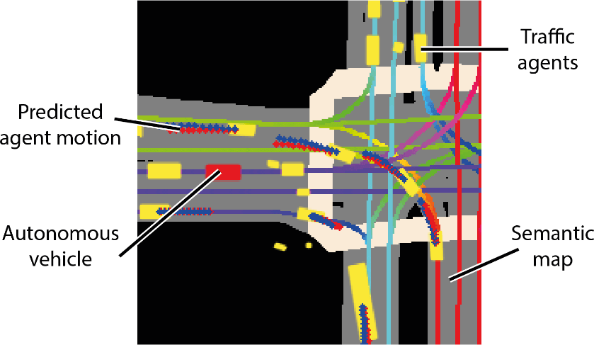
Lyft used a fleet of cars equipped with LIDARs and cameras to collect a large dataset. They were driving along the streets of Palo Alto and scanned the environment around the cars.
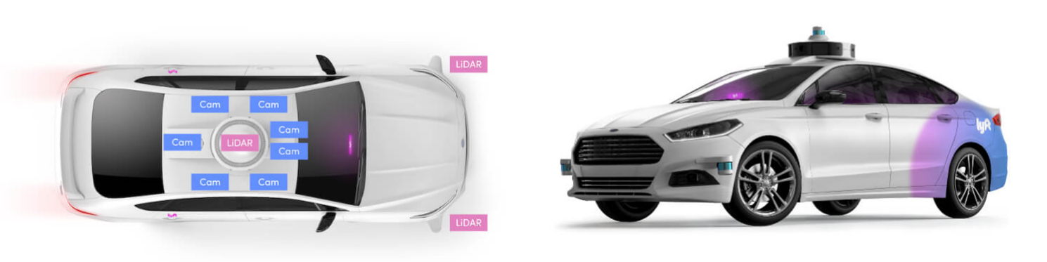
The LIDARs and cameras were used to obtain 3D point clouds which were then processed to detect all the surrounding objects (other cars, pedestrians, cyclists, road signs, and so on). Then Lyft engineers registered objects on the map using GPS and the corresponding 3D coordinates.
They record a lot of trips to cover very diverse road situations. The collected dataset (Houston et al., 2020) contains more than 1000 hours of driving in total.
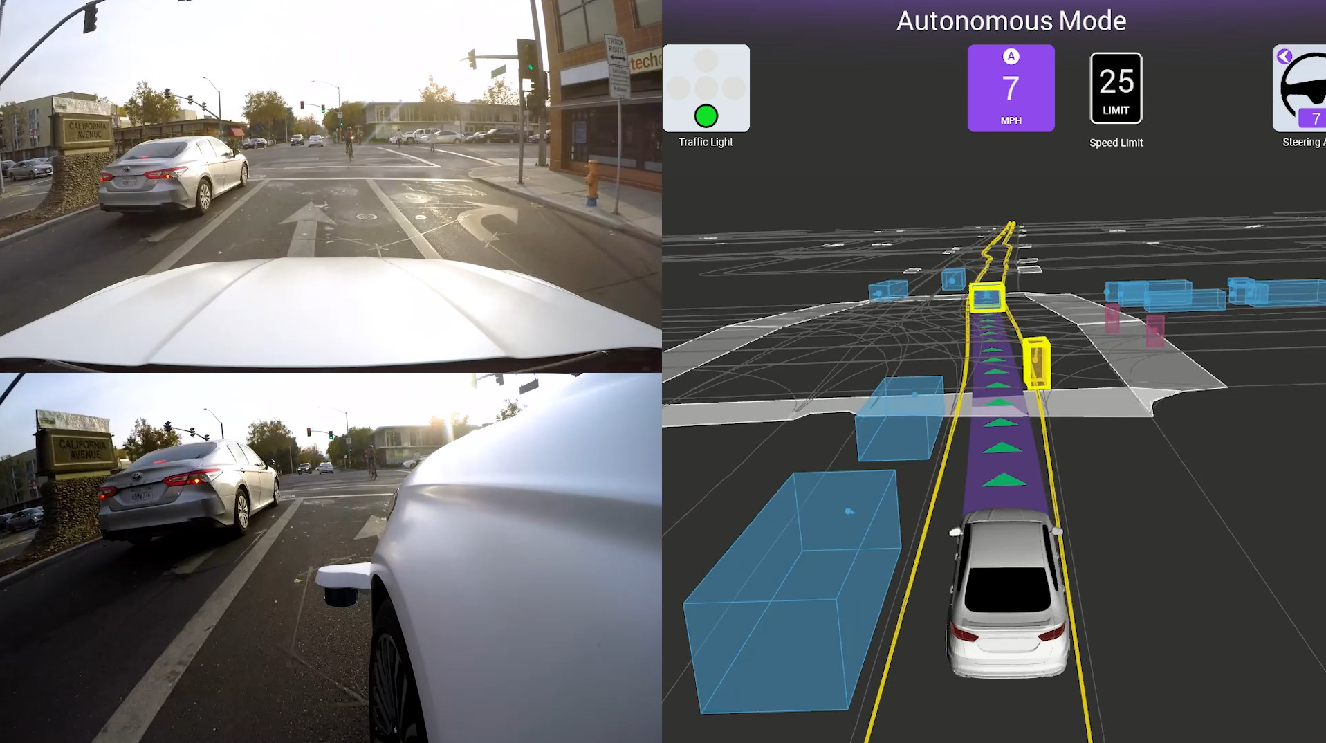
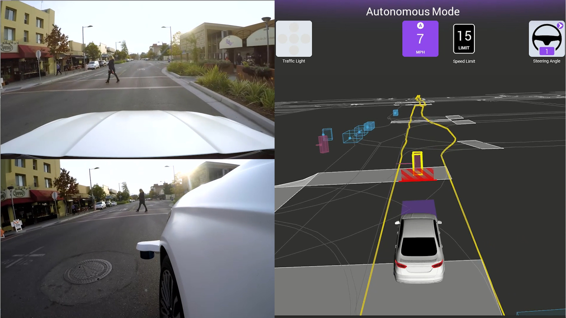
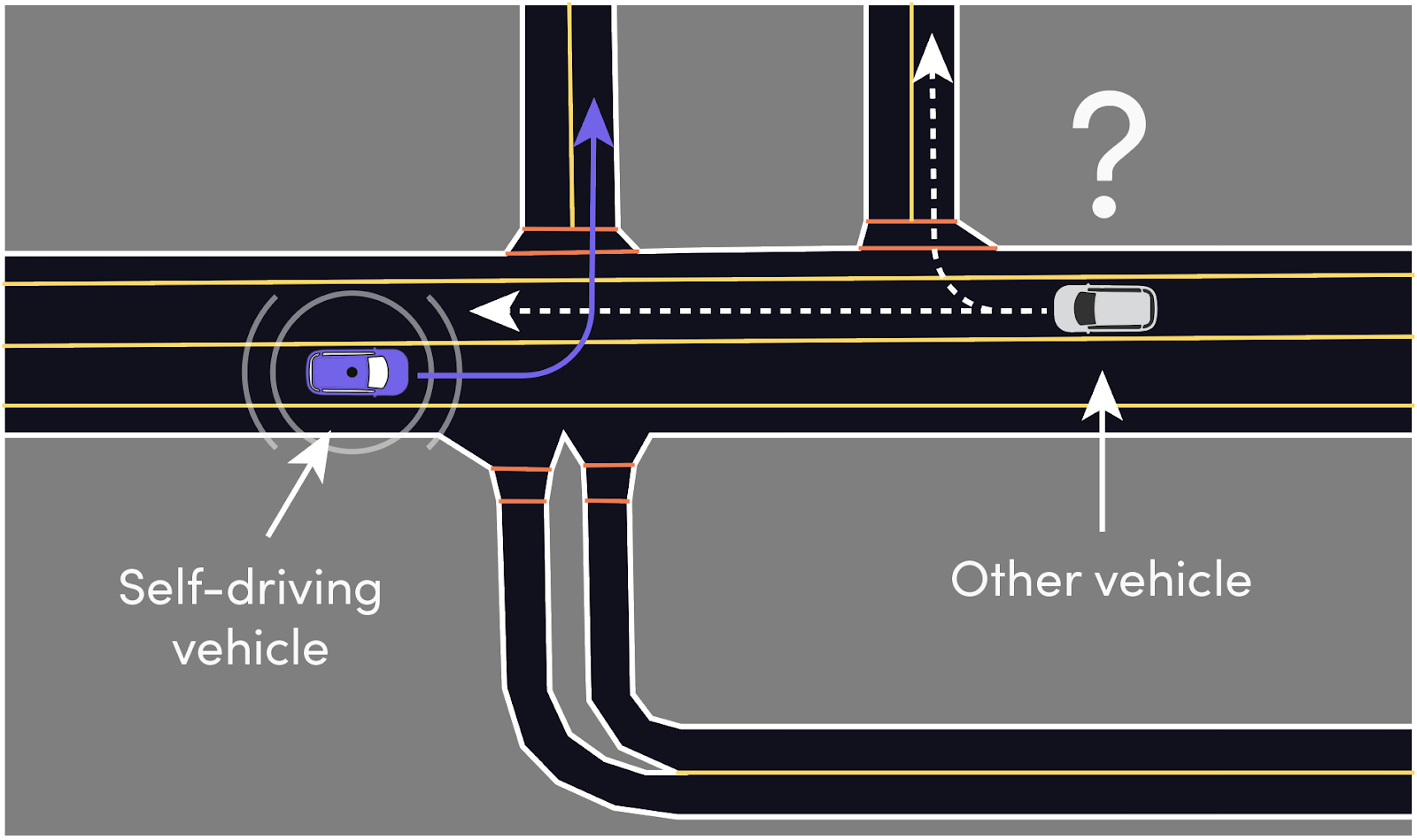
As you can see in the Figure above the perception task is pretty much solved and the current Lyft pipeline shows fairly robust results. However, for an autonomous vehicle (AV) to correctly plan its future actions, it needs to know what to anticipate from other agents nearby (e.g., other cars, pedestrians, and cyclists).
Future motion prediction along with the AV's route planning are still very challenging problems and are yet to be solved for the general case.
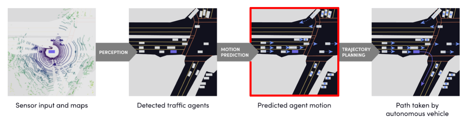
In this competition we had to tackle the motion prediction task.
Input Data and Evaluation Metric
We are given a travel history of the agent and its current location on the map which was collected as we described in the previous section. For every agent we have from 0 to 50 history snapshots with a time interval of 0.1 seconds. So our input can be represented as an image with \(3 + (50 + 1) * 2 = 105\) channels. Here first 3 channels is the RGB map. Then we have 50 history time steps and one current. Every time step is represented by two channels: (1) The mask representing the location of the current agent, and (2) the mask representing all other agents nearby.
The task is to predict the trajectory of the agent for the next 50 time steps in future.
Kaggle test server allowed to submit 3 hypothesis (proposals) for the future trajectory which were compared with the ground truth trajectory. The evaluation metric of this competition - negative log-likelihood (NLL) of the ground truth coordinates in the distribution defined by the predicted proposals. The lower the better. In other words, given the ground truth trajectory \(\text{GT}\) and \(K\) predicted trajectory hypotheses \(\text{hypothesis}_k, k=1,...,K\), we compute the likelihood of the ground truth trajectory under the mixture of Gaussians with the means equal to the predicted trajectories and the Identity matrix as a covariance.
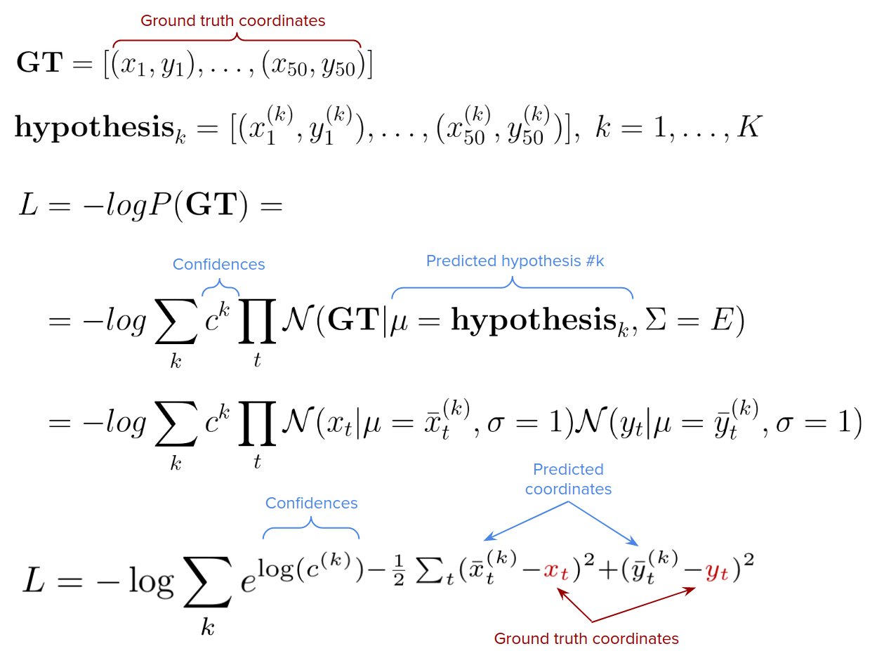
For every hypothesis we provide a confidence value \(c^{(k)}\), such that \(\sum_k c^{(k)} = 1\). This metric can be further decomposed into the product of 1-dimensional Gaussians, and we get just a log sum of the exponents. Note that in the evaluation metric we ignore the constant normalizing factors of the Gaussian distributions.
Method
Model
In practice, it is usually a good idea to optimize directly the target metric if possible. So, for the training loss, we used the same function as the evaluation metric (see image above).
What you always should do in any Kaggle competition first - is to start with a simple baseline model.
Our baseline is a simple CNN with one fully-connected layer which takes an input image with \(C\) channels and predicts \(3\) trajectories with the corresponding confidences.
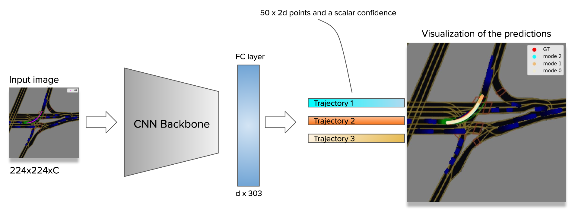
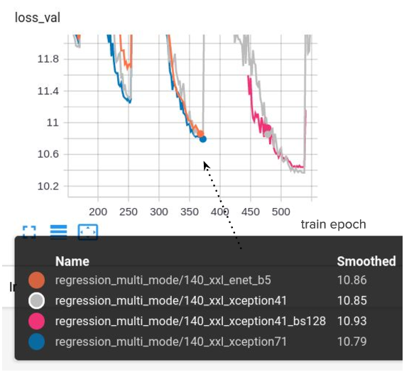
And it turned out that this simple baseline model worked the best for us. It became the core of our solution. Of course, following the common practice, we experimented with different CNN backbones. Among the best performing backbones were Xception41, Xception65, Xception71, and EfficientNet B5.
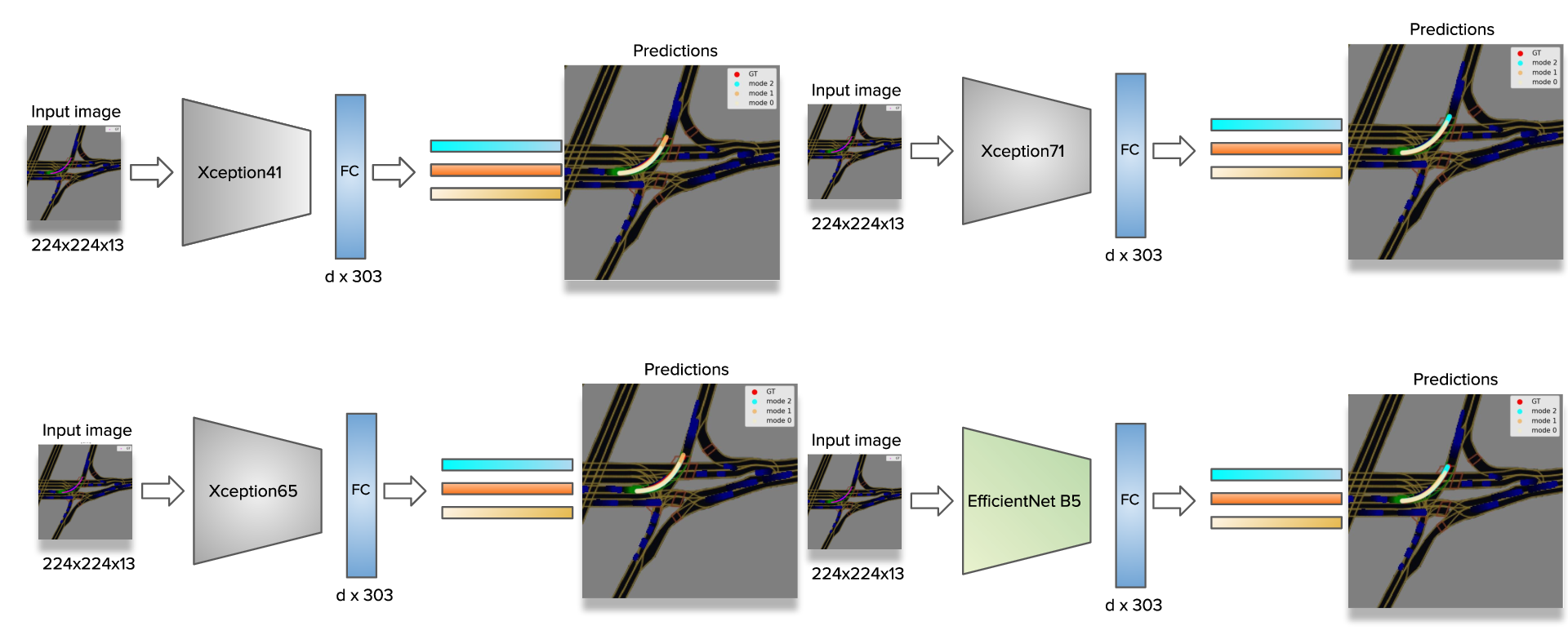
Unfortunately, we didn’t have time to train all the models until convergence. Given the limited time and resources, the model with Xception41 as a backbone showed the best performance: validation score of 10.37, which is in the range of 5-6th places at the public Leaderboard. Training for longer (especially the model with Xception71 backbone) is likely to improve the score. We observed that our validation scores had a very strong correlation with the scores on the public test set, but usually were lower on some fixed constant.
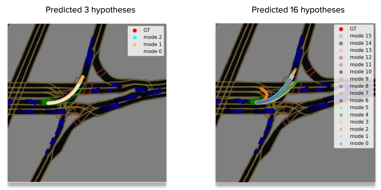
Beyond the models with \(3\) output trajectories, we also trained a model with \(16\) hypotheses which resulted in more diverse predictions.
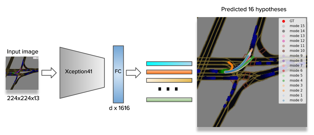
For example, both left turn and U-turn are plausible in the situation on the image and the \(16\)-output model predicts these in contrast to the previous model with \(3\) outputs.
Ensemble learning
Model ensembling is a very powerful technique. Ensembles combine multiple hypotheses (generated by a set of weaker models) to form a (hopefully) better hypothesis. We ensembled 7 different models. Six models with 3 output trajectories:
- Xception41 backbone (x3 different):
- batch size 64
- batch size 128
- weighted average pooling (similar to average pooling but uses learnable weights instead of fixed uniform weights)
- Xception65
- Xception71
- EfficientNetB5
And one Xception41 model with 16 output hypotheses.
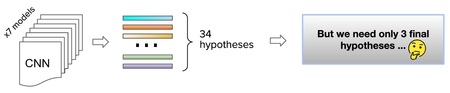
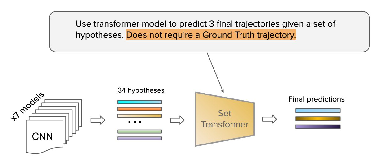
By running inference on all these models we got in total \(6 \times 3 + 1 \times 16 = 34\) hypotheses and their corresponding confidences. But we can submit only 3 final hypotheses for evaluation.
One of the biggest challenges of this competition is how to combine multiple hypotheses in order to produce only 3 required for the evaluation.
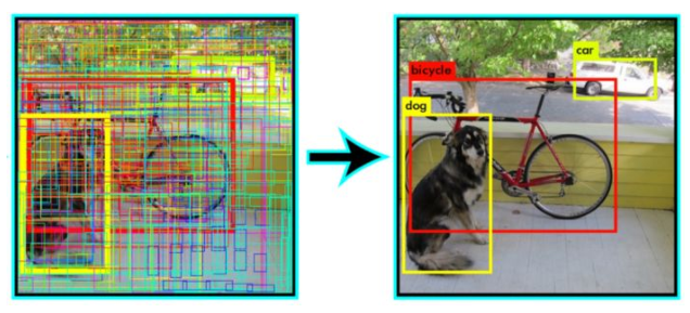
Obviously, it is beneficial to select \(3\) very diverse proposals as it increases the chance that one of them will be close to the Ground Truth. One can see that such a problem statement is closely related to a well known Non-maximum suppression method widely used in object detection pipelines, where multiple spurious detections have to be filtered.
A trivial way to do Non-maximum suppression is a greedy algorithm. We iteratively select the most confident detection while suppressing very similar but less confident ones.
We applied a similar greedy approach to our task as well. At every step we selected the most confident trajectory and suppressed very similar ones (those which have very small Euclidean distance between one another). However, this greedy algorithm didn’t work well for our task and gave worse results than the best Xception41 model with 3 hypotheses.
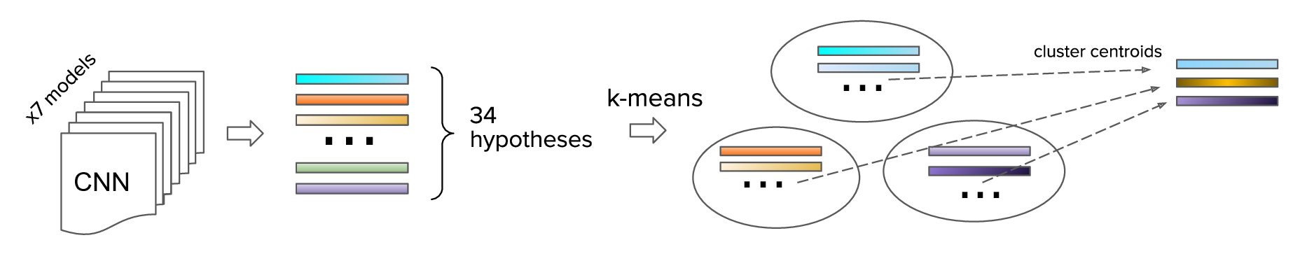
We tried another approach. We applied K-means clustering with 3 clusters to the pool of 34 hypotheses and used their centroids as the final predictions. However, this didn’t work well either. Another attempt was to compute a weighted average of the clusters using the confidences as weights. Unfortunately, neither of these methods could outperform the best single model with the Xception41 backbone. We speculate that the discrete nature of greedy non-maximum suppression and K-means significantly limits the possible solution space.
To combat this shortcoming we considered an extension of the non-maximum suppression to the continuous case. And these naturally led us to the Gaussian Mixture Model (GMM). We fit a mixture of 3 Gaussians to the pool of the hypotheses and used the obtained means of the Gaussians as the final predictions.
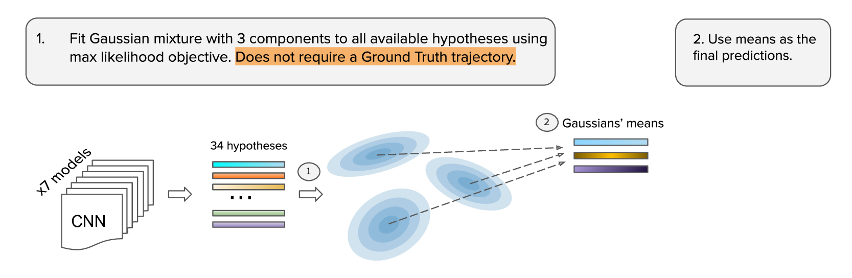
The optimized objective is very similar to the traditional Gaussian Mixture model objective. It is the log-likelihood of the input hypotheses. The only modification to the original Gaussian Mixture Model objective is that every hypothesis is weighted according to its confidence.
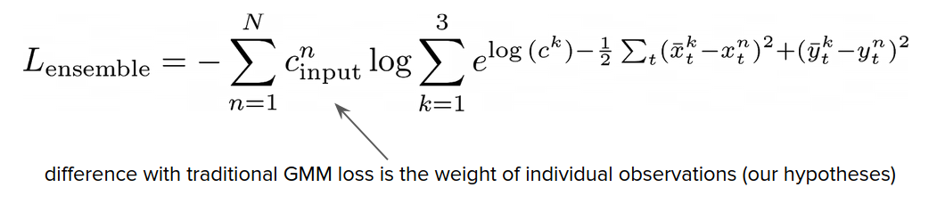
We can optimize this objective using Gradient Descent or Expectation-Maximization (EM) algorithm. This approach works pretty well and produces a solution better than any single model in the ensemble, but it can easily get stuck in local optima and is very sensitive to the initialization.
To further improve the results we implemented a Neural Network model which optimizes this loss and can produce a solution in a single forward pass.
The important property which we require of this neural network is to be permutation invariant for input hypotheses, because hypotheses produced by CNN models do not have any particular order.
In other words, a neural network has to take a set of hypotheses as input and produce 3 final trajectories. As the model satisfying our needs we selected Set Transformer.
Set Transformer has an encoder that takes input hypotheses and their confidences and applies two self-attention blocks to them to produce feature vectors that encode all pairwise relations between the input hypotheses. Next, the first block of the decoder takes 3 learnable seed vectors which represent the prototypes for our three output trajectories, and attend to the most relevant representations of the input hypotheses from the encoder, next follows another self-attention block after which we produce 3 output trajectories and the corresponding confidences.
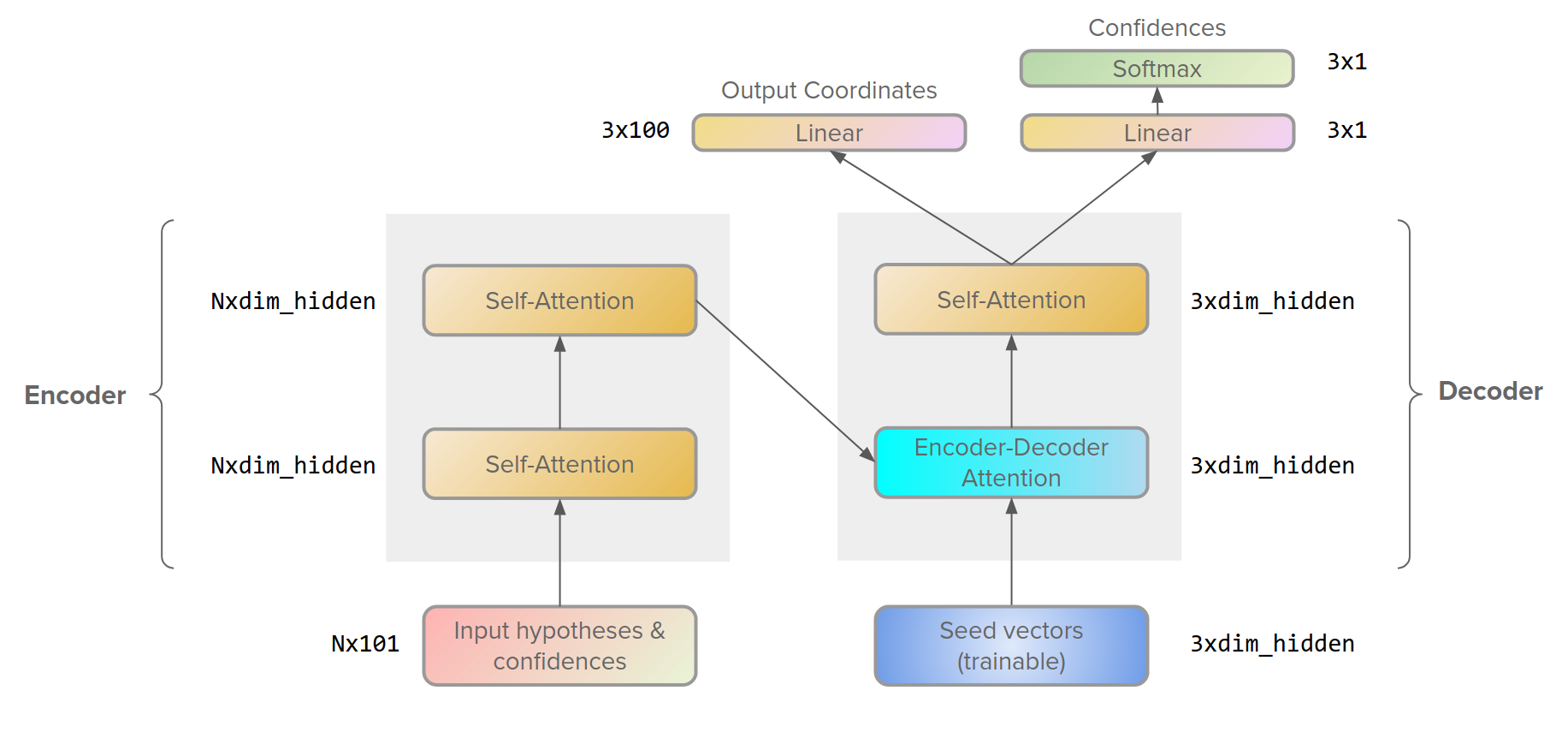
This Transformer is invariant to the permutation of the input trajectories and it does not utilize positional encoding. Essentially, it takes a lot of trajectories as inputs and outputs 3 new ones that describe the input in the best possible way. Such a model can leverage global statistics of the entire training dataset, whereas Gaussian mixture and clustering do not have a global context and work sample-wise.
Training details
In this competition, it was crucial to find a proper learning rate schedule. We used SGD with a relatively high learning rate of 0.01, batch size 64 (if not stated otherwise), and a Cosine Annealing scheduler with warm restarts. The first cycle length was 50.000 iterations, and we increased the length of every next cycle by a factor of \(\sqrt{2}\). Another important trick was gradient clipping (maximal magnitude was set to 2) which stabilized training, especially at the initial epochs.
Significant score improvement was achieved after we allowed training samples to be without history at all (before that they were ignored). Such examples can be often encountered in the real-life test when a previously unseen car approaches the AV and the model has to predict the future motion of that car relying merely on its prior knowledge about other road agents. Utilizing such examples increased the training complexity and improved the model generalization to validation and test sets.
We trained each model for around a week on a single GPU of Titan XP / GTX 2080Ti level. Longer training may bring even better results.
Rasterizer parameters and optimization
To generate the training images from raw data, we used the rasterizer provided by Lyft in the package l5kit. We used default rasterization parameters and produced images of \(224 \times 224\) pixels.
One of the major speed bottlenecks in the pipeline was image rasterization.
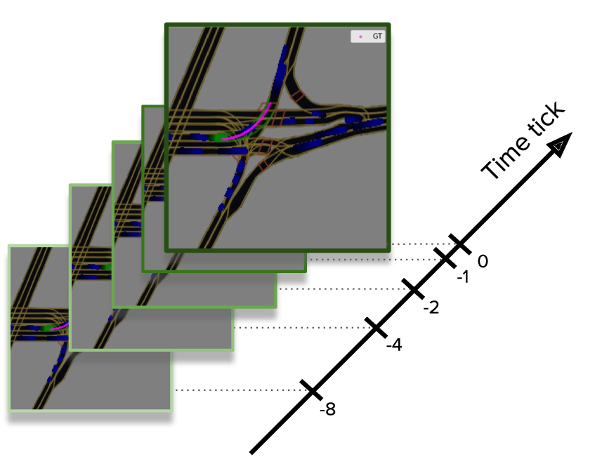
Important detail which improved our training efficiency is using a sparse set of only 4 history time steps instead of maximum allowed 50 steps. We used only 1, 2, 4, and 8 ticks in the past. We did not notice any improvement in the target metric score when we used more history steps.
The default l5kit rasterizer is pretty slow (even with the sparse set of history steps) and produces around 15 images per second on a single CPU core. To make training faster we optimized the rasterizer. First, we uncompressed z-arr files that contained raw data and combined multiple operations like a transformation of points into numba optimized functions. This gave almost x2 speedup. Then, we cached the rasterized images to disk as compressed npz files. And during training we just loaded them from disk instead of costly online rasterization. This resulted in x7 speedup and we could read more than a hundred images per second using a single process.
Another important step was to start using the entire dataset which contains more than 1000 hours of driving which is almost 9 times larger than the subset originally provided at Kaggle.
The full dataset is huge and it has been taking days to finish a single training epoch on it.
However, the dataset is redundant in the sense that consecutive frames (time difference between them is 0.1 sec) are highly correlated. To allow the model to see more various road situations in a fixed amount of time we removed highly correlated samples by selecting only every 8th frame for every agent in the dataset (subsampling in time with the step of 0.8 seconds). This significantly reduced the epoch training time as well as the disk space required for caching the dataset (from 10 TB to 1.3 TB).
Experiments
Ablation studies
We conducted ablation studies on one of the intermediate ensemble (before the models converged).
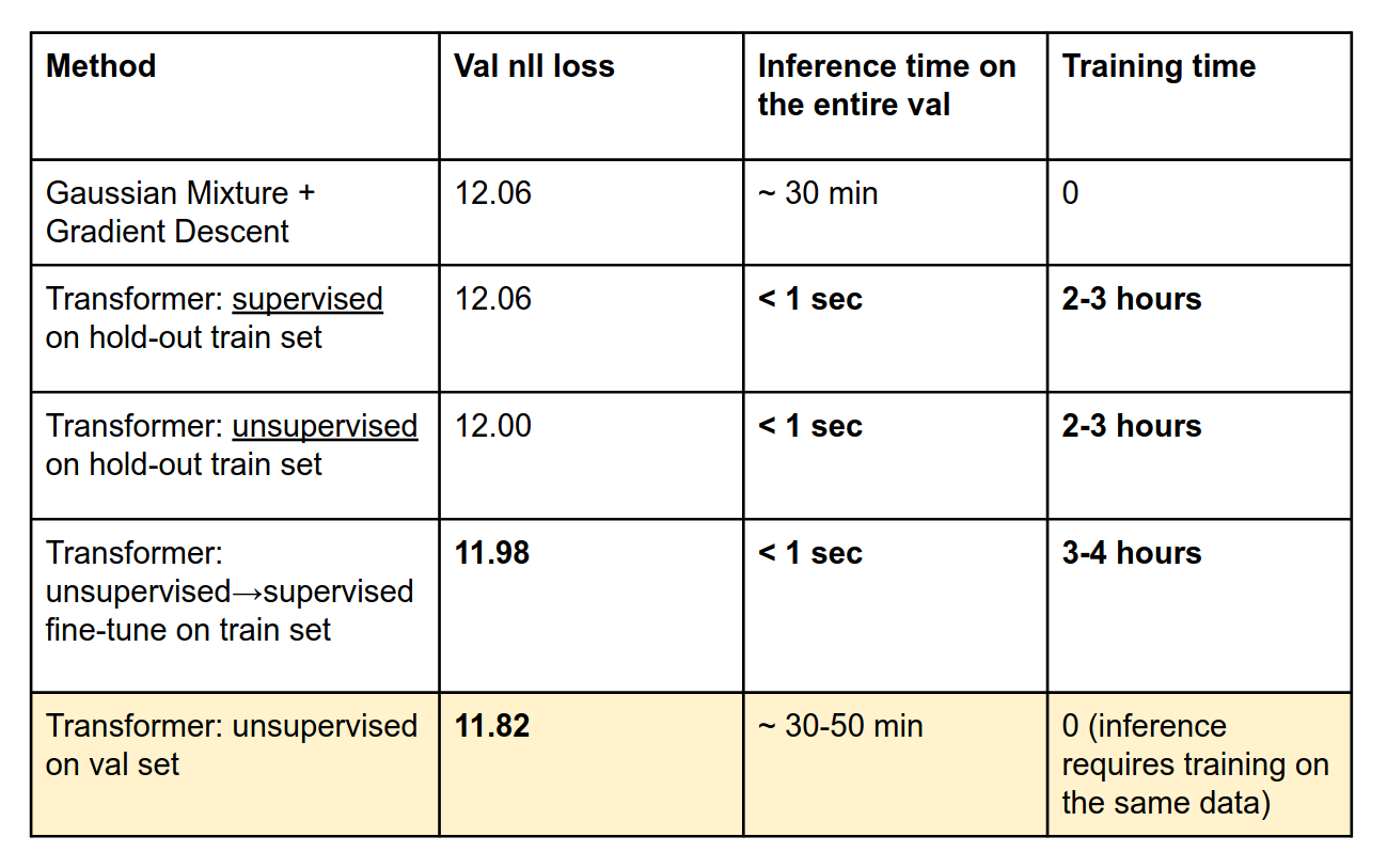
Our transformer can also be trained in a supervised fashion, using the same loss which we used for our first level CNN models. I.e., transformer predicts three trajectories, and the negative log-likelihood loss (NLL) is computed using these three predictions and the ground truth trajectory. To prevent data leak we trained this transformer on a hold-out set from the “full train dataset”. In this case, the transformer performs on par with the Gaussian mixture (12.06 validation loss). However, the transformer is faster during inference because it requires only a single forward pass while the Gaussian Mixture involves a costly optimization process.
Surprisingly, unsupervised training of the transformer on the hold-out training set which doesn’t require GT trajectories performs better than the supervised (12.00 vs 12.06). We speculate that the reason for this is that it is hard for the model to learn to produce diverse outputs with supervised loss when most of the hypotheses are too far from the GT trajectory. In this case, the diversity of the output is highly penalized which hinders the model performance.
We also tried to pre-train the transformer in an unsupervised way and then finetune using the supervised loss. This brought a small improvement by 0.02 (from 12.00 to 11.98).
Finally, we trained the set transformer directly in the validation set in an unsupervised way (i.e. without using GT trajectories). This way we achieved the best validation score of 11.82.
Final results
In this table we present our final results.
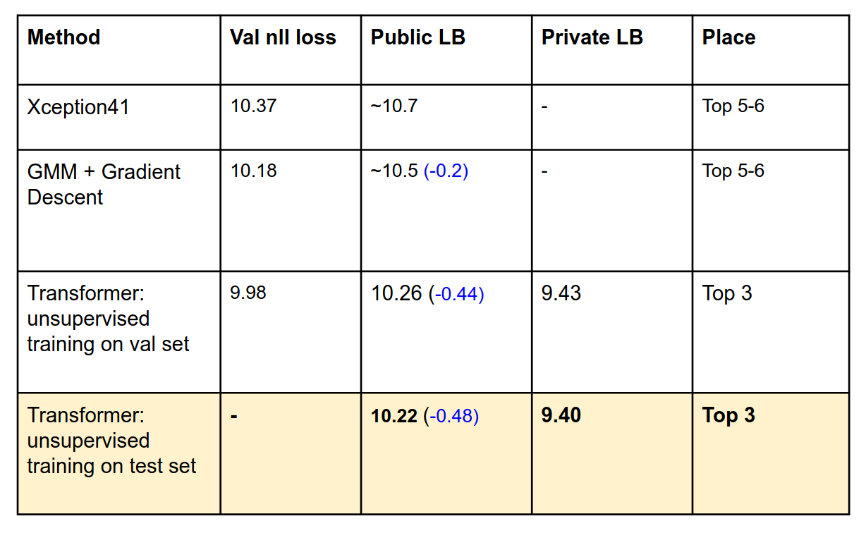
The Set Transformer model trained on the test set directly (without using GT of course) is superior to all other models. However, it requires retraining for every novel piece of data and maybe less suitable for production than a Transformer pretrained on a hold-out set. In contrast, transformer pretrained on some large hold-out set is very quick for inference on new observations but is slightly less accurate.
Conclusion
- A simple CNN regression baseline turned out to be the best model and very hard to beat (as always keep it simple).
- Training for longer with the right parameters on the entire dataset was crucial.
- It was very important to optimize the rasterizer to train faster.
- Ensembling with Set Transformer can be used for model ensembling and it lifted our team to 3rd place.
- Unsupervised training of the model directly on the test data yields the best performance. However, if the test data arrives continuously in time, such a model would need to be re-trained for every new chunk of data.
Solution source code and model weights: GitHub repo.
Video explanation of the solution: video.
This article can be cited as:
@article{sanakoyeu2021lyft,
  title   = "Winning Solution for Kaggle Challenge: Lyft Motion Prediction for Autonomous Vehicles.",
  author  = "Sanakoyeu, Artsiom and Dmytro Poplavskiy and Artsem Zhyvalkouski",
  journal = "gdude.de/blog",
  year    = "2021",
  url     = "https://gdude.de/blog/2021-02-05/Kaggle-Lyft-solution"
}
Feel free to ask me any questions in the comments below. Feedback is also very appreciated.
- Join my telegram channel for more reviews like this
 @gradientdude
 - Follow me on twitter
 @artsiom_s