Multi-Animal Linear model (SMAL): Modeling the 3D Shape and Pose of Animals
“3D Menagerie: Modeling the 3D Shape and Pose of Animal”, Zuffi et al, CVPR 2017.
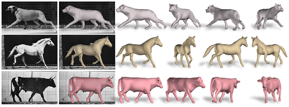
Fig. 1: Predicted animal 3D shapes from images. (Image source: Zuffi et al, CVPR 2017)
We will discuss the method which allows to create a realistic 3D model of animals and to fit this model to 2D images [Arxiv PDF].
Main contribution:
- Global/Local Stitched Shape model (GLoSS) which aligns a template mesh to different shapes, providing a coarse registration between very different animals.
- Multi-Animal Linear model (SMAL) which provides a shape space of animals trained from 41 scans
- the model generalizes to new animals not seen in training
- one can fit SMAL to 2D data using detected keypoints and binary segmentations
- SMAL can generate realistic animal shapes in a variety of poses.
Method
Dataset
The authors collected a dataset of 3D animals by scanning toy figurines.
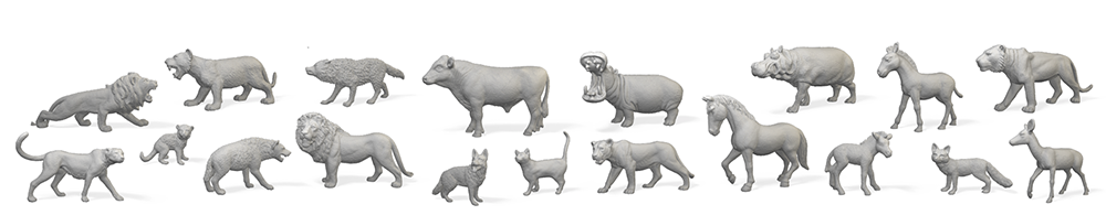
Fig. 2: Examples of collected 3D scans of animal toys. (Image source: Zuffi et al, CVPR 2017)
A total of 41 scans from several species: 1 cat, 5 cheetahs, 8 lions, 7 tigers, 2 dogs, 1 fox, 1 wolf, 1 hyena, 1 deer, 1 horse, 6 zebras, 4 cows, 3 hippos. For every 3D scans authors manually annotated 36 semantically-aligned keypoints.
1. Aligning, rigging, and parametrizing the training 3D scans by matching them with GLoSS model
The aim is to learn a parametric model from a set of training 3D scans, that covers all training shapes, generalizes to the shape of animals not seen during training, and can be fitted to the images of real animals.
To learn such a model one needs to align all the training 3D scans and make them articulated by rigging.
This is a hard problem, which we authors approach by introducing a novel part-based reference model (GLoSS) and inference scheme that extends the “stitched puppet” (SP) model [1].
The Global/Local Stitched Shape model (GLoSS) is a 3D articulated model where body shape deformations are locally defined for each part and the parts are assembled together by minimizing a stitching cost at the part interfaces. To define GloSS authors do:
- Select a 3D template mesh of some animal
- Manually segment it into 33 body parts
- Define skinning weights.
- Get an animation sequence of this model using linear blend skinning (LBS).
For this purpose authors used an off-the-shelf 3D mesh of a lioness which is already rigged and has predefined skinning weights.
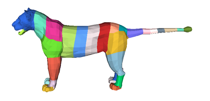
Fig. 3: 3D template mesh of a lioness used for GLoSS. Color denotes manually segmented 33 body parts. (Image source: Zuffi et al, CVPR 2017)
To get the pose deformation space for GloSS, the authors perform PCA on the vertices of each frame in the animated 3D sequence.
To get the shape deformation space for GLoSS: authors model scale and stretch deformations along x,y,z axes for each body part using a Gaussian distribution.
After that, we can fit GLoSS model to every 3D scan from the training set using the gradient-based methods.
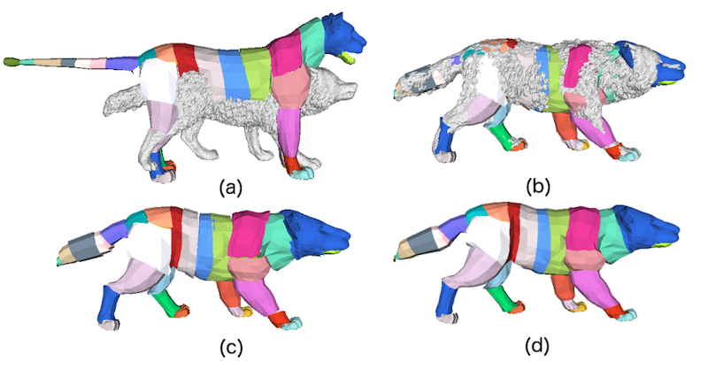
Fig. 4: GLoSS fitting. (a) Initial template and scan. (b) GLoSS fit to scan. (c) GLoSS model showing the parts. (d) Merged mesh with global topology obtained by removing the duplicated vertices. (Image source: Zuffi et al, CVPR 2017)
To bring the mesh vertices closer to the scan authors further align the vertices v of the model to the scans using the As-Rigid-As-Possible (ARAP) method [2].
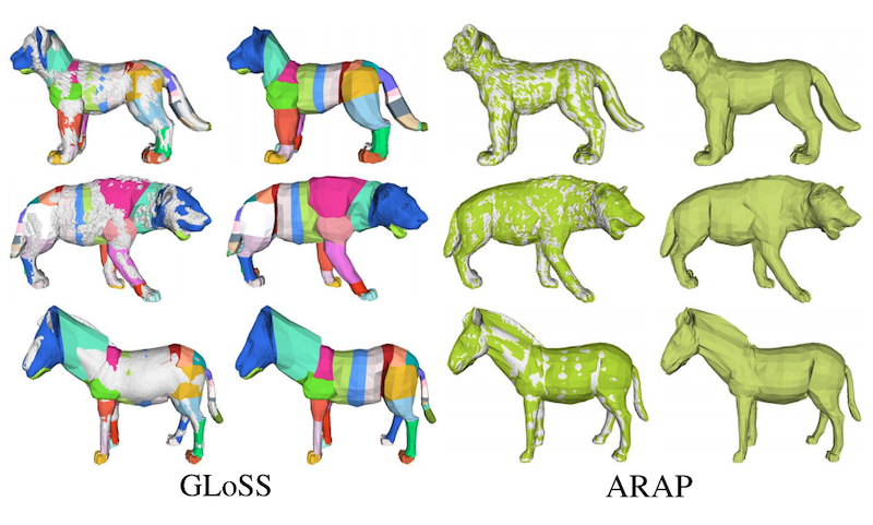
Fig. 5: Registration results. Comparing GLoSS (left) with the ARAP refinement (right). The fit to the scan is much tighter after refinement. (Image source: Zuffi et al, CVPR 2017)
2. Learning parametric SMAL model
Now, given the poses estimated with GLoSS, authors model shape variation across training dataset by
- Bringing all the registered templates into the same neutral pose using LBS;
- Learn shape space by computing the mean shape and the principal components (PCA), which capture shape differences between the animals.
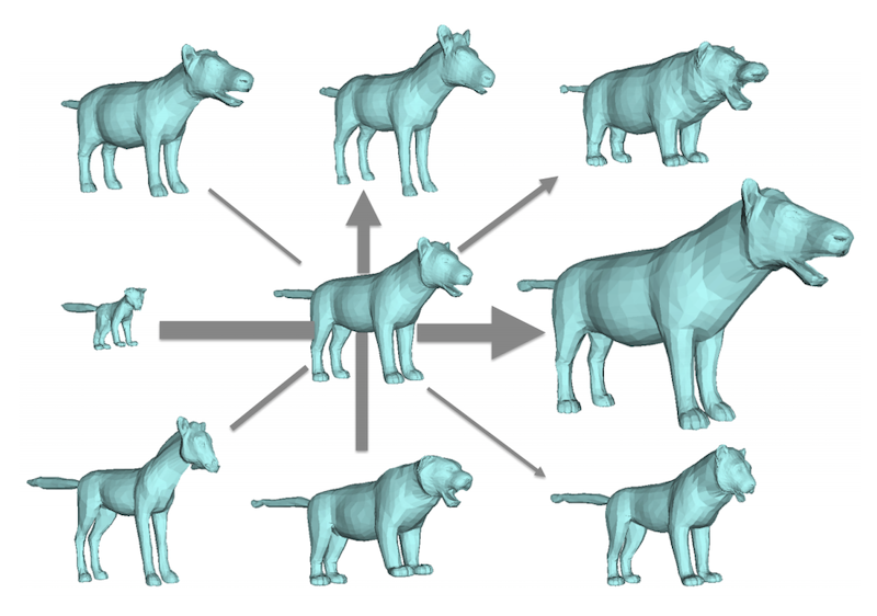
Fig. 6: Visualization of the mean shape (in the center) and the variation along the first 4 components of the learned shape PCA space. (Image source: Zuffi et al, CVPR 2017)
SMAL is then a function which is parametrized by shape, pose, and translation parameters. The output of SMAL is a 3D mesh.
3. How to fit SMAL to a 2D image?
Given an input image with an animal, first, we need to manually annotate (or predict with another CNN) 36 keypoints and a binary foreground mask (silhouette). We fit the SMAL model to the image by fitting its parameters and camera pose using the keypoints and silhouette reprojection error.
Reprojection error is computed by rendering the estimated SMAL mesh, projecting it on the input image, and comparing the predicted keypoints and silhouette with those defined on the input image. The local optimum is found by iterative optimization. Optimization for a single image typically takes less than a minute.
Results
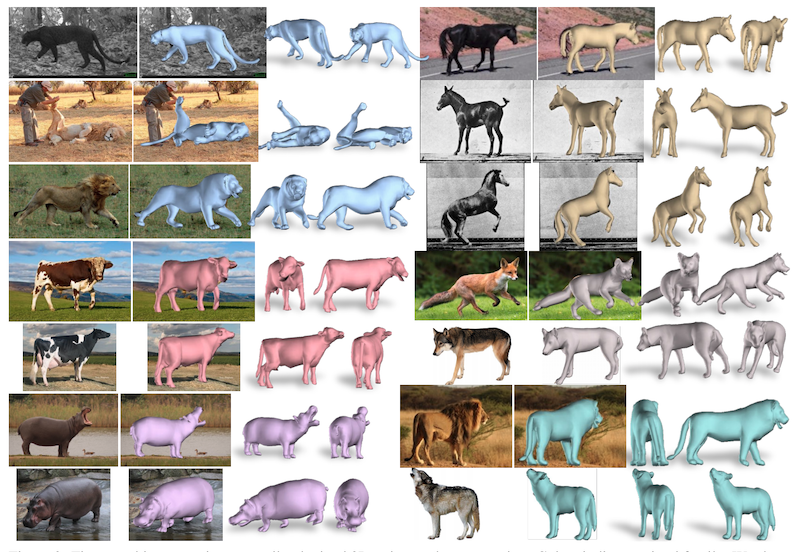
Fig. 7: Results of the SMAL model fit to real images using manually obtained 2D keypoints and segmentation. (Image source: Zuffi et al, CVPR 2017)
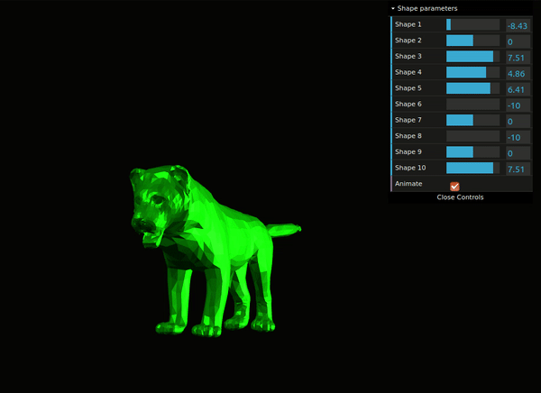
Fig. 8: Interactive demo of SMAL model.
You can explore a web-demo which allows you to interactively change the SMAL shape parameters and see how the output mesh transforms (Fig. 8).
More results can be found at http://smal.is.tuebingen.mpg.de/.
Conclusion
Authors showed that starting with toys’ 3D scans, we can learn a model that generalizes to images of real animals as well as to types of animals not seen during training. The proposed parametric SMAL model is differentiable and can be fit to the data using gradient-based algorithms.
References
[1] The stitched puppet: A graphical model of 3D human shape and pose, Zuffi et al. CVPR 2015.
[2] As-Rigid-As-Possible Surface Modeling, Sorkine et al., Symposium on Geometry Processing, 2007.
Feel free to ask me any questions in the comments below. Feedback is also very appreciated.
- Join my telegram channel for more reviews like this
 @gradientdude
 - Follow me on twitter
 @artsiom_s